I recently acquired a FLIR ONE thermal camera, which deserves a separate post reviewing it, but for now let’s look at the TP4056 Li-Ion charger with integrated protection circuitry.
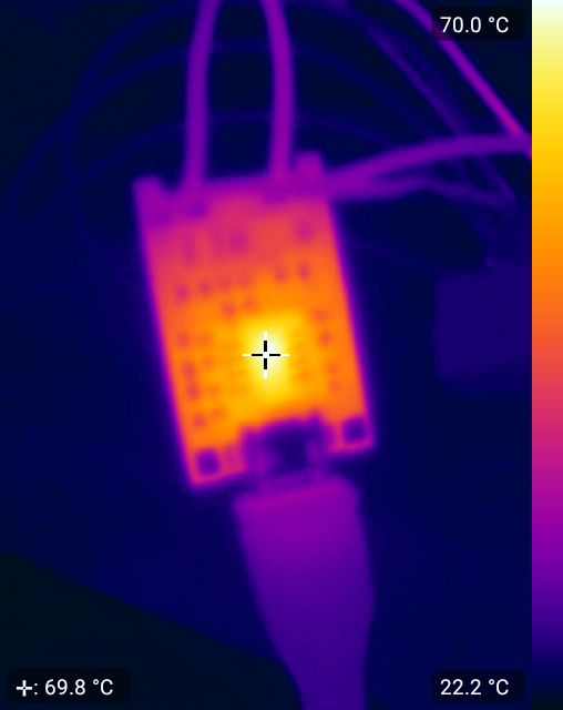
This is a pretty bog-standard, dirt-cheap Li-Ion charger that works really well. It does what it says on the tin: CC/CV charging, with charging current adjustable by replacing a specific resistor, 5V MicroUSB input, and pads/holes to accept connections to the cell, the load, and the charging power source (if one doesn’t want to use the USB port). No complaints at all, and no surprises.I like that it has a battery protection circuit as well: the protection chip monitors the charging or discharging current and voltage, and protects the cell against overvoltage (e.g. from over-charging), undervoltage (e.g. from over-discharging), and over-current situations by switching off the MOSFET that connects the battery to the load and charging chip.The FET is arranged in a cool way such that, even if the over-discharge protection has tripped and the FET is open, you can trickle charge through the FET’s body diode at a very low rate in order to slowly charge the cell up without stressing it. Once it reaches the release voltage, the cell will charge at the normal speed.One of the main reasons I bought the FLIR ONE thermal camera is to observe various electronic devices I have and see how hot they get, where the heat is dissipated, etc. Since the TP4056 is a linear charger and produces a modest amount of heat while charging, I figured this would make a great first test. Here’s one of the images I snapped:
As you can see, the chip gets moderately toasty when charging at 1A, and I can’t hold my finger on it for a more than a second or two. This is a top view with the chip and other components visible to the camera. The TP4056 also has a thermal “radiator” (using the language in the datasheet) pad on the bottom that should be connected to a copper plane on the PCB. The board has a bunch of thermal vias under the chip to conduct the heat away to the other side and the backside of the board is about the same temperature as the front. Neat.
I foresee a lot of fun (and useful projects) with both the camera and the battery charger.
Thermocouples are amazing temperature sensors. They’re simple (just two wires!), cover a wide range of temperatures, have no moving parts, are incredibly robust, and are easy to use and deploy.
However, the temperature-dependent voltage they produce is very small (for example, the common K-type I refer to throughout this post produces a nominal 41.276μV/°C) and they require temperature compensation if their “cold junction” (the end not being used to measure something and which is not necessarily colder than the sensing end) is not at exactly 0°C, so purpose-built chips like the MAX31855 are made to amplify the very weak signal, measure the cold junction temperature and apply the necessary compensation, digitize the readings, and provide the result over a digital interface like SPI.
However, the MAX31855 has one glaring issue: it assumes the temperature-to-voltage relationship (the “characteristic function”) of the thermocouple is linear over its entire -200°C to +1,350°C temperature range. It isn’t.
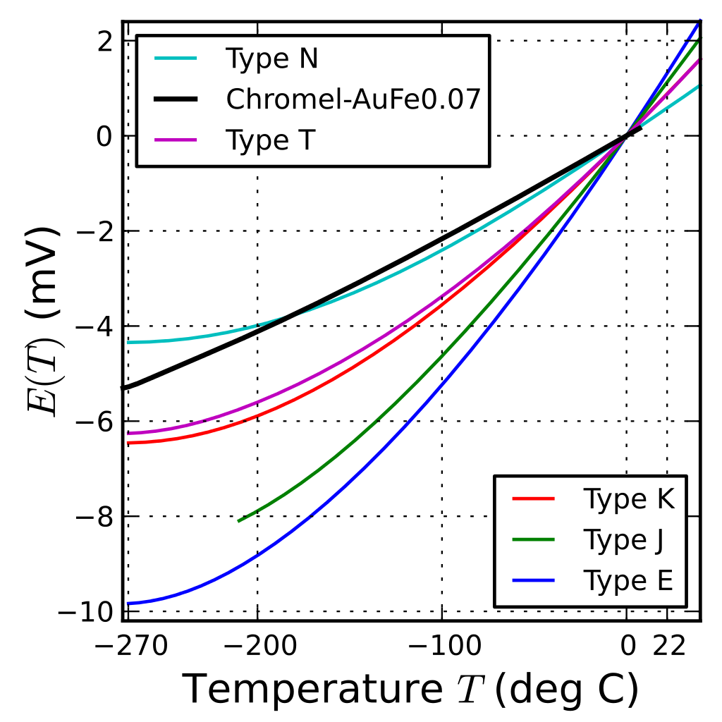
In fact, for K-type thermocouples, the characteristic function goes highly non-linear at very low temperatures. Ideally, E(-100°C) would be -4.128mV. Instead, it’s -3.554mV according to the NIST tables. E(-200°C) should ideally be -8.256mV, but it’s actually -5.891mV. Yikes!
Characteristic function for selected thermocouple types at low temperatures.
At positive temperatures, K-type thermocouples are significantly more linear, with <1% error at 1,000°C and ~2.2% at 1,350°C. Although the MAX31855 works across the full range of temperatures for K-type thermocouples, it’s obviously designed to be mainly used in the linear, positive-temperature territory.
Part of my work involves measuring things at both liquid nitrogen temperatures (-195°C) and at very high temperatures (200-1,000°C). I can tolerate an error of a few degrees, but when I immersed a type-K thermocouple in liquid nitrogen and connected it to a MAX31855, the reported temperature was only -130°C.
Not good.
Fortunately, the good folks at Maxim Integrated provided me with a handy guide on how to properly correct the non-linearized output of the MAX31855. It’d be easy if the chip would provide us the actual thermocouple voltage it measured, but it doesn’t (darn!), so we need to reverse to calculations it does internally to derive the measured voltage so we can apply the corrections.
Let’s walk through how to do so in 5 easy steps. We’ll use the example values from the guide: the true temperature being measured is -99.16°C, the cold junction temperature is 22.9375°C, and the non-linearized cold junction-compensated temperature (“raw”, using the guide’s term) output by the MAX31855 is -84.75°C.
First, subtract the cold junction temperature from the raw temperature:-84.75°C – 22.9375°C = -107.6875°C
Next, calculate the thermocouple voltage corresponding to that temperature if we assume the thermocouple was perfectly linear and E(T) was 0.041276mV/°C:-107.6875°C * 0.041276mV/°C = -4.44490925mV
This part’s a bit tricky: we need to calculate the equivalent thermocouple voltage (“E”, in mV) of the cold junction using the cold junction temperature reading from the MAX31855, the NIST temperature-to-voltage coefficients (c0, c1, …, cn and a0, a1, and a2). The an values are only used for positive temperatures. For some reason, Maxim uses different letters for the coefficients than NIST, so keep that in mind. Here’s the formulas we need:For temperatures <0°C:$latex E = \sum\limits_{i=0}^10 c_i \cdot t^i$For temperatures >0°C:$latex E = \sum\limits_{i=0}^9 c_i \cdot t^i + a_0 \cdot e^{\left(a_1 \left(t – a_2\right)\right)^2}$
Where t is the temperature of the cold junction. The coefficients are different for positive and negative temperatures, so be sure you’re using the right values from the table.
The example in the guide has the cold junction near room temperature, so we need to use the equation for positive temperatures. I’m rounding the coefficients here for readability, but you should use the full ones in your code.
The next step is easy: just add the cold junction equivalent thermocouple voltage you calculated in step 3 to the thermocouple voltage calculated in step 2:-4.44490925mV + 0.916753mV = -3.528157mV
The result of step 4 is the linearized thermocouple voltage. Now we just need to convert that voltage to a temperature. Fortunately, NIST has done the hard work for us and provided us with an easy equation:$latex T = d_0 + d_1 \cdot E + d_2 \cdot E^2 + d_3 \cdot E^3 + … + d_n \cdot E^n$, where T is the corrected, linearized temperature in °C, dn are the inverse coefficients given at the bottom of NIST tables (note: there’s three groups of inverse coefficients, each corresponding to a different temperature and voltage range — be sure to use the right one!), and E is the sum of the two thermocouple voltages you calculated in step 4.$latex 0 + \left(2.52 \times 10^{1} \cdot -3.528157\right) + \left(-1.17 \times 10^{2} \cdot -3.528157^2\right) + \left(-1.08 \times 10^{3} \cdot -3.528157^3\right) + … + \left(-5.19 \times 10^{8} \cdot -3.528157^8\right) = -99.16^{\circ}\textrm{C}$
That’s it!
I’ve put up some MIT-licensed example Arduino code at my GitHub repository that will perform the necessary corrections. It uses the Adafruit MAX31855 library to talk to the chip, though it should be easy enough to adapt if you’re not using that library or are developing for another platform. Any suggestions or improvements are welcome!
Fellow Adafruit forum member jh421797 has also made some handy code for accomplishing the same result. It, as well as an earlier version of my code (my GitHub repo has the latest version), is available on the Adafruit site.
Fortunately, Maxim has now released a worthy successor to this chip: the MAX31856 improves on the MAX31855 by adding 50/60Hz line frequency filtering to remove noise induced by power lines, a 19-bit (vs 14-bit for the MAX31855) analog-to-digital converter, support for many different types of thermocouples using a single chip (vs needing to buy a different chip for different types), and, critically, automatic linearization using an internal lookup table.
Interfacing with the MAX31856 is slightly different than the MAX31855, but Peter Easton has released an excellent Arduino library for it. He also makes and sells excellent, US-made breakout boards for the MAX31856 in both 5V and 3.3V editions. I highly recommend them. (Full disclosure: he sold me a few at a discounted rate for testing and evaluation. See my brief review here.)